It is critical for the foundation of the aquatic food web, for the condition of the environment and the biodiversity of the ocean, for fisheries and many activities at sea. A more realistic representation of the Eastern Boundary Upwelling Systems (EBUS) variability at interannual to decadal scale is provided by a study led by scientists at the CMCC Foundation and published on Nature Scientific Reports.

Upwelling is a process in which deep, cold water rises toward the surface. Typically, water that rises to the surface as a result of upwelling is colder and rich in nutrients. This is the reason why coastal upwelling ecosystems are some of the most productive ecosystems in the world and support many of the world’s most important fisheries.
For example, the Eastern Boundary Upwelling Systems (EBUS), such as the California Current System (CalCS), the Canary Current System (CanCS), the Humboldt Current System (HCS), and the Benguela Current System (BenCS), are among the most productive marine ecosystems, supplying up to 20% of the global fish catches, although they only cover approximately 1% of the total ocean. Surface alongshore winds, force the offshore water transport and the divergence of the surface flow, thereby lifting nutrient-rich deep waters into the euphotic layer. The nutrient-rich upwelled water, in addition to the sunlight, sustains the blooms of phytoplankton that are the foundation of the aquatic food web.

Understanding the drivers and monitoring changes across EBUS is becoming increasingly important: many studies have in fact documented trends and changes at decadal scale in the EBUS ecosystem structure. Coastal warming increases the water stratification and it might limit the effectiveness of upwelling to bring nutrient-rich deep waters up to the surface. Increasing or decreasing of the upwelling-favourable winds might also mitigate or amplify the effect of coastal warming. Coastal waves may also influence the water column stratification modulating coastal biogeochemical conditions and triggering vertical displacements of the thermocline, which controls subsurface anomalies (e.g., salinity), and thus the impact on EBUS productivity.
Moreover, we have to mention the influence of the main large-scale ocean-atmosphere processes: the El Niño Southern Oscillation (ENSO), the Pacific Decadal Oscillation (PDO), the North Pacific Gyre Oscillation (NPGO), the North Atlantic Oscillation (NAO), the Atlantic Multidecadal Oscillation (AMO) seem to play a role in controlling the upwelling variability.

A study published on Nature Scientific Reports was aimed at understanding the coherent and non-coherent low frequency variability across the EBUS, and to explore how it is linked to large-scale climate modes, with the aim of modelling and studying the interannual to decadal variability of the major Eastern Boundary Upwelling Systems. The study, led by scientist Giulia Bonino, researcher at the CMCC ODA – Ocean modeling and Data Assimilation Division, and co-authored by CMCC scientists Simona Masina and Dorotea Iovino, and by Emanuele Di Lorenzo from Georgia Institute of Technology, focuses on quantifying forcing dynamics (e.g. alongshore winds, wind stress curl, thermocline depth) that controls low-frequency modulations in each EBUS while aiming at identifying how the forcing is linked to large-scale climate dynamics, to finally understand the extent to which large-scale climate dynamics imprint a coherent signal across EBUS.

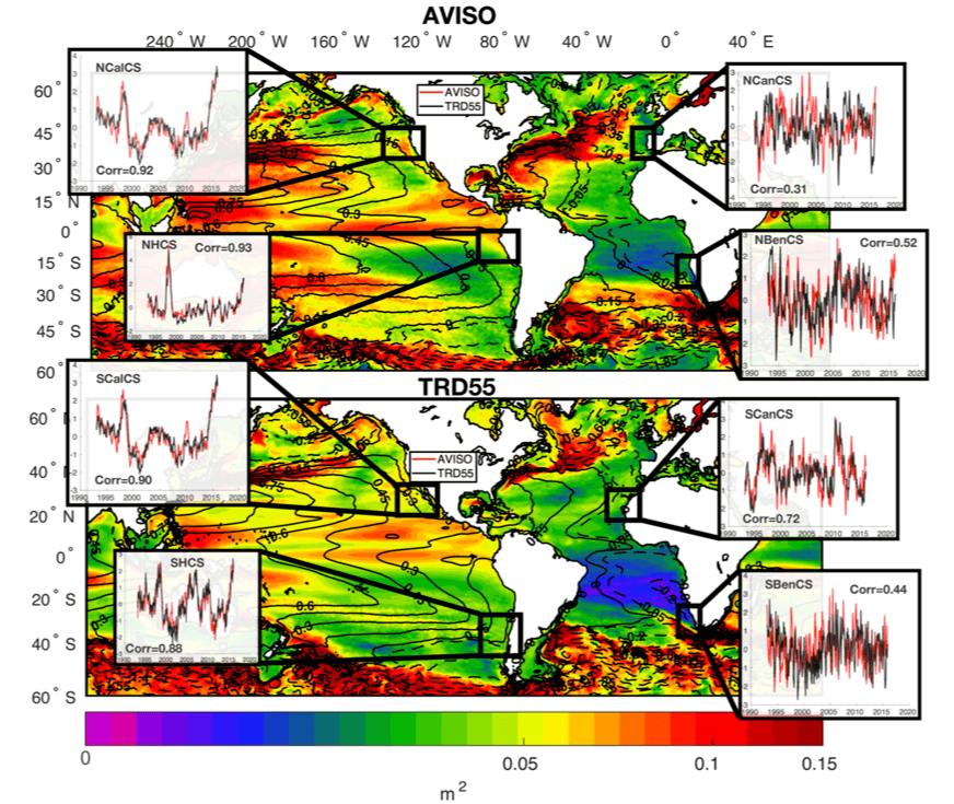
Figure 1: SSHa standard deviation (shaded areas) and mean SSHa (contour), from satellite altimetry data (AVISO, top panel) and model solution (TRD55, bottom panel) during 1993–2015 period; subplots: normalized SSHa from AVISO data and model solution during 1993–2015 period.

Researchers modelled ocean dynamics in upwelling areas using a global eddy-permitting configuration of the NEMO model from 1958 to 2015. To quantify the upwelling, they introduced an ensemble of passive tracers in the simulation, which are continuously released in the subsurface layer (150–250 m) in each EBUS over a region from the coast to 50 km offshore.
“The results highlight the uniqueness of each EBUS in terms of drivers and climate variability”, explains Giulia Bonino. “The local (e.g., wind forcing, stratification and thermocline depth) and the remote (e.g. passage of coastal trapped waves) forcing, with different contribution in each EBUS, appear to control the interannual upwelling variability. Thus, in order to predict and to propose hypotheses on the long-term variations in upwelling, identifying a proper index of upwelling in relation to the major drivers of each domain is essential. In particular, both the coastal wind variations and the stratification have to be considered as potentially competitive or complementary drivers of upwelling variability under climate change.”

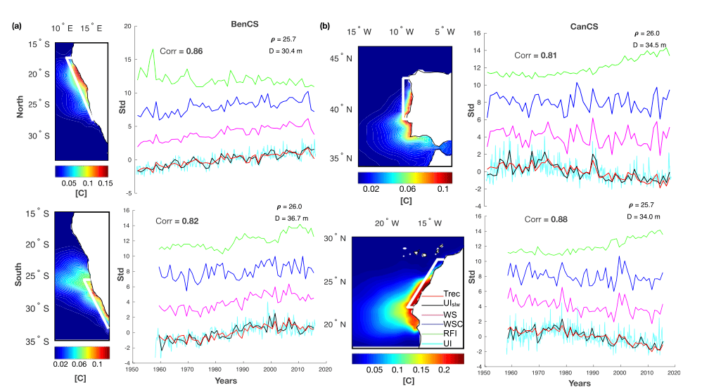
Figure 2: For (a) Benguela and (b) Canary systems: Long-term mean (1958–2015) of surface passive tracers concentration (left panels); low-frequency modulation of upwelling (UIslw, black line), alongshore wind stress (WS, purple line), wind stress curl (WSC, blue line) and RFI (RFI, green line) seasonal cycle and the reconstructed times series of upwelling using the above mentioned timeseries as drivers (Trec, red line) (right panels). In cyan monthly time series of tracer anomaly (UI). Corr indicates the correlation between predicted and reconstructed time series.

The second important issue addressed in the study is the influence of the large-scale climate variability on long-term upwelling and the degree to which there is coherent low-frequency variability across EBUS. “The variability associated with climate modes could be of importance to predict future perturbations at interannual to decadal time scales”, explains Giulia Bonino. “Our results show that signs of global warming, characterized by strong upwelling winds in a changing climate, are evident only over the Benguela system. From a broader climate prospective, EBUS do not share variability, except from the well-known influence of ENSO on the Pacific systems. Therefore, Atlantic and Pacific upwelling systems appear to be independent. Extending the current analysis to a longer period, with coupled models and with the same passive tracers approach, will help to clarify these issues, enabling the results to be compared, and to confirm any unexpected teleconnections between upwelling systems.”

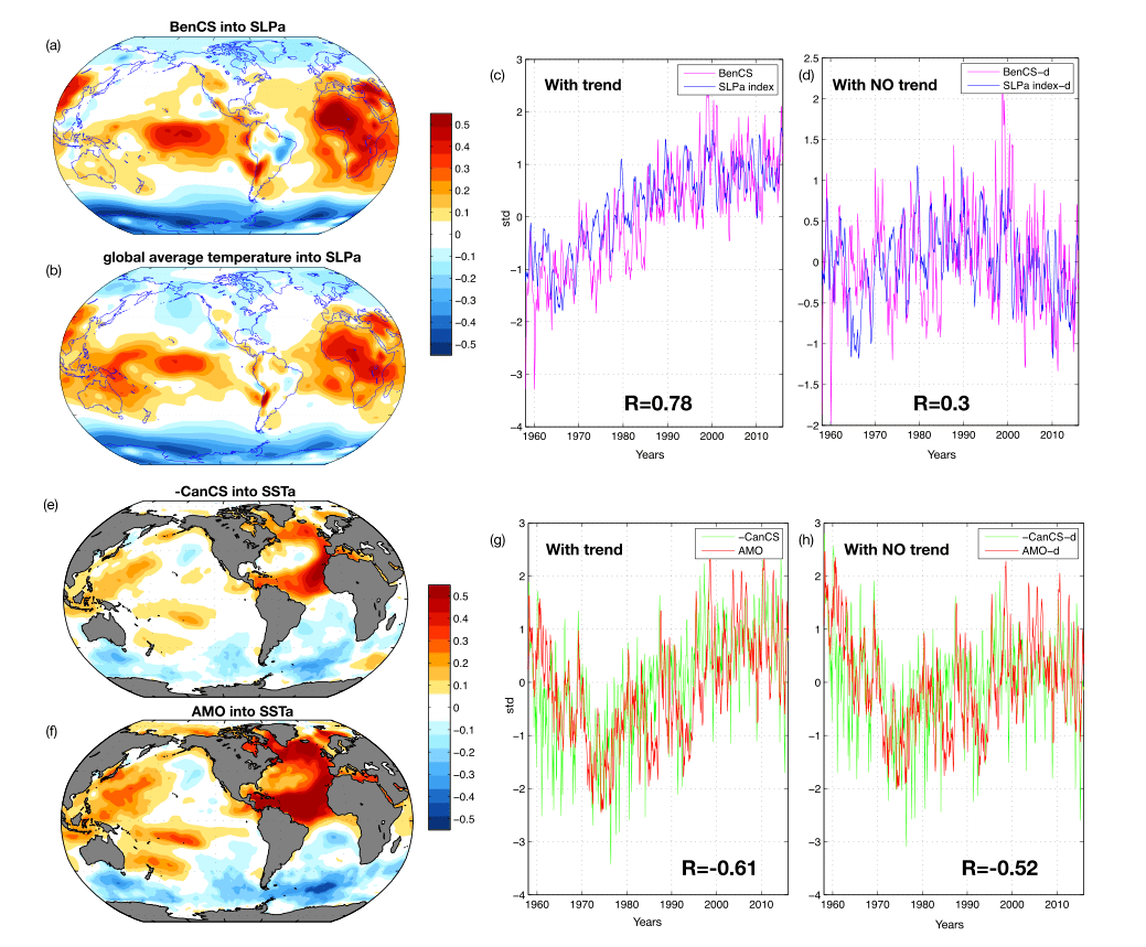
Figure 3: (a) Correlation pattern between Benguela Current System upwelling (BenCS UI) and Sea Level Pressure (NCEP SLPa); (b) Correlation patterns between NOAA global average temperature (1958–2015) and NCEP SLPa; (c) BenCS UI and SLPa index (climate change proxy); (d) detrended BenCS and detrended SLPa index (climate change proxy). -d identifies detrended indices, R identifies significant correlation coefficients; (e) Correlation patterns between -CanCS UI and NOAA SSTa; (f) Correlation pattern between AMO index and NOAA SSTa; (g) -CanCS UI and AMO index; (h) detrended -CanCS UI and detrended AMO index. -d identifies detrended indices, R identifies significant correlation coefficients.

See all the figures of this study here.

Read more:
The paper on Nature Scientific Reports:
Bonino, G., Di Lorenzo, E., Masina, S. et al. Interannual to decadal variability within and across the major Eastern Boundary Upwelling Systems. Sci Rep 9, 19949 (2019). https://doi.org/10.1038/s41598-019-56514-8